
Book Contents
Overview: This is an introductory text on the science (and art) of image processing. The book employs the Matlab programming language and toolboxes to illuminate and consolidate some of the elementary but yet key concepts in modern image processing and pattern recognition.
For most of us, it is through good examples and gently guided experimentation that we really learn. Accordingly, the book has a large number of carefully chosen examples, graded exercises and computer experiments designed to help the reader get a real grasp of the material. All the program code (.m files) used in the book, corresponding to the examples and exercises, are made available to the reader/course instructor and may be downloaded from the materials section of this site.
Sample Material: [Chapter 1] [
Index] [
Wiley On-line Library] [
Google Books Preview]
(PDFs as provided by the publisher
here.
These samples are copyright and may not be re-produced.)
Independent Reviews: [
IAPR Newsletter] [
BMVA News] [
Blackwells] [
Amazon CA]
Table of Contents
-
Chapter 1: Representation
(materials)

- 1.1 What is an image?
- 1.1.1 Image layout
- 1.1.2 Image colour
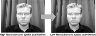
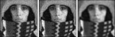
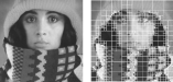
- 1.2 Resolution and quantization
- 1.2.1 Bit-plane splicing
- 1.3 Image formats
- 1.3.1 Image data types
- 1.3.2 Image compression
- 1.4 Colour spaces
- 1.4.1 RGB
- 1.4.1.1 RGB to grey-scale image conversion
- 1.4.2 Perceptual colour space
- 1.5 Images in Matlab
- 1.5.1 Reading, writing and querying images
- 1.5.2 Basic display of images
- 1.5.3 Accessing pixel values
- 1.5.4 Converting image types
- 1.1 What is an image?
-
Chapter 2: Formation
(materials)
- 2.1 How is an image formed?
- 2.2 The mathematics of image formation
- 2.2.1 Introduction
- 2.2.2 Linear imaging systems
- 2.2.3 Linear superposition integral
- 2.2.4 The Dirac delta or impulse function
- 2.2.5 The point-spread function
- 2.2.6 Linear shift-invariant systems and the convolution integral
- 2.2.7 Convolution: its importance and meaning
- 2.2.8 Multiple convolution: N imaging elements in a linear shift-invariant system
- 2.2.9 Digital convolution
- 2.3 The engineering of image formation
- 2.3.1 The camera
- 2.3.2 The digitization process
- 2.3.2.1 Quantization
- 2.3.2.2 Digitization hardware
- 2.3.2.3 Resolution versus performance
- 2.3.3 Noise
-
Chapter 3: Pixels
(materials)
- 3.1 What is a pixel?
- 3.2 Operations upon pixels
- 3.2.1 Arithmetic operations on images
- 3.2.1.1 Image addition and subtraction
- 3.2.1.2 Multiplication and division
- 3.2.2 Logical operations on images
- 3.2.3 Thresholding
- 3.2.1 Arithmetic operations on images
- 3.3 Point-based operations on images
- 3.3.1 Logarithmic transform
- 3.3.2 Exponential transform
- 3.3.3 Power-law (gamma) transform
- 3.3.3.1 Application: gamma correction
- 3.4 Pixel distributions: histograms
- 3.4.1 Histograms for threshold selection
- 3.4.2 Adaptive thresholding
- 3.4.3 Contrast stretching
- 3.4.4 Histogram equalization
- 3.4.4.1 Histogram equalization theory
- 3.4.4.2 Histogram equalization theory: discrete case
- 3.4.4.3 Histogram equalization in practice
- 3.4.5 Histogram matching
- 3.4.5.1 Histogram-matching theory
- 3.4.5.2 Histogram-matching theory: discrete case
- 3.4.5.3 Histogram matching in practice
- 3.4.6 Adaptive histogram equalization
- 3.4.7 Histogram operations on colour images
-
Chapter 4: Enhancement
(materials)
- 4.1 Why perform enhancement?
- 4.1.1 Enhancement via image filtering
- 4.2 Pixel neighbourhoods
- 4.3 Filter kernels and the mechanics of linear filtering
- 4.3.1 Nonlinear spatial filtering
- 4.4 Filtering for noise removal
- 4.4.1 Mean filtering
- 4.4.2 Median filtering
- 4.4.3 Rank filtering
- 4.4.4 Gaussian filtering
- 4.5 Filtering for edge detection
- 4.5.1 Derivative filters for discontinuities
- 4.5.2 First-order edge detection
- 4.5.2.1 Linearly separable filtering
- 4.5.3 Second-order edge detection
- 4.5.3.1 Laplacian edge detection
- 4.5.3.2 Laplacian of Gaussian
- 4.5.3.3 Zero-crossing detector
- 4.6 Edge enhancement
- 4.6.1 Laplacian edge sharpening
- 4.6.2 The unsharp mask filter
- 4.1 Why perform enhancement?
-
Chapter 5: Linear systems and frequency-domain processing
(materials)
- 5.1 Frequency space: a friendly introduction
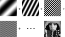
- 5.2 Frequency space: the fundamental idea
- 5.2.1 The Fourier series
- 5.3 Calculation of the Fourier spectrum
- 5.4 Complex Fourier series
- 5.5 The 1-D Fourier transform
- 5.6 The inverse Fourier transform and reciprocity
- 5.7 The 2-D Fourier transform
- 5.8 Understanding the Fourier transform: frequency-space filtering
- 5.9 Linear systems and Fourier transforms
- 5.10 The convolution theorem
- 5.11 The optical transfer function
- 5.12 Digital Fourier transforms: the discrete fast Fourier transform
- 5.13 Sampled data: the discrete Fourier transform
- 5.14 The centred discrete Fourier transform
-
Chapter 6: Image restoration
(materials)
- 6.1 Imaging models
- 6.2 Nature of the point-spread function and noise
- 6.3 Restoration by the inverse Fourier filter
- 6.4 The Wiener–Helstrom Filter
- 6.5 Origin of the Wiener–Helstrom filter
- 6.6 Acceptable solutions to the imaging equation
- 6.7 Constrained deconvolution
- 6.8 Estimating an unknown point-spread function or optical transfer function
- 6.9 Blind deconvolution
- 6.10 Iterative deconvolution and the Lucy–Richardson algorithm
- 6.11 Matrix formulation of image restoration
- 6.12 The standard least-squares solution
- 6.13 Constrained least-squares restoration
- 6.14 Stochastic input distributions and Bayesian estimators
- 6.15 The generalized Gauss–Markov estimator
-
Chapter 7: Geometry
(materials)
- 7.1 The description of shape
- 7.2 Shape-preserving transformations
- 7.3 Shape transformation and homogeneous coordinates
- 7.4 The general 2-D affine transformation
- 7.5 Affine transformation in homogeneous coordinates
- 7.6 The Procrustes transformation
- 7.7 Procrustes alignment
- 7.8 The projective transform
- 7.9 Nonlinear transformations
- 7.10 Warping: the spatial transformation of an image
- 7.11 Overdetermined spatial transformations
- 7.12 The piecewise warp
- 7.13 Linear, piecewise affine warp
- 7.14 Warping: forward and reverse mapping
-
Chapter 8: Morphological processing
(materials)

- 8.1 Introduction
- 8.2 Binary images: foreground, background and connectedness
- 8.3 Structuring elements and neighbourhoods
- 8.4 Dilation and erosion
- 8.5 Dilation, erosion and structuring elements within Matlab
- 8.6 Structuring element decomposition and Matlab
- 8.7 Effects and uses of erosion and dilation
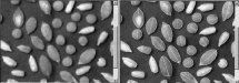
- 8.7.1 Application of erosion to particle sizing
- 8.8 Morphological opening and closing
- 8.8.1 The rolling-ball analogy
- 8.9 Boundary extraction
- 8.10 Extracting connected components
- 8.11 Region filling
- 8.12 The hit-or-miss transformation
- 8.12.1 Generalization of hit-or-miss
- 8.13 Relaxing constraints in hit-or-miss: ‘don’t care’ pixels
- 8.13.1 Morphological thinning
- 8.14 Skeletonization
- 8.15 Opening by reconstruction
- 8.16 Grey-scale erosion and dilation
- 8.17 Grey-scale structuring elements: general case
- 8.18 Grey-scale erosion and dilation with flat structuring elements
- 8.19 Grey-scale opening and closing
- 8.20 The top-hat transformation
-
Chapter 9: Features
(materials)

- 9.1 Landmarks and shape vectors
- 9.2 Single-parameter shape descriptors
- 9.3 Signatures and the radial Fourier expansion
- 9.4 Statistical moments as region descriptors
- 9.5 Texture features based on statistical measures
- 9.6 Principal component analysis
- 9.7 Principal component analysis: an illustrative example
- 9.8 Theory of principal component analysis: version 1
- 9.9 Theory of principal component analysis: version 2
- 9.10 Principal axes and principal components
- 9.11 Summary of properties of principal component analysis
- 9.12 Dimensionality reduction: the purpose of principal component analysis
- 9.13 Principal components analysis on an ensemble of digital images
- 9.14 Representation of out-of-sample examples using principal component analysis
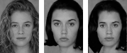
- 9.15 Key example: eigenfaces and the human face
-
Chapter 10: Image Segmentation
(materials)
- 10.1 Image segmentation
- 10.2 Use of image properties and features in segmentation
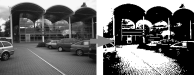
- 10.3 Intensity thresholding
- 10.3.1 Problems with global thresholding
- 10.4 Region growing and region splitting
- 10.5 Split-and-merge algorithm
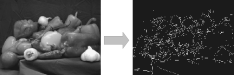
- 10.6 The challenge of edge detection
- 10.7 The Laplacian of Gaussian and difference of Gaussians filters
- 10.8 The Canny edge detector
- 10.9 Interest operators
- 10.10 Watershed segmentation
- 10.11 Segmentation functions
- 10.12 Image segmentation with Markov random fields
- 10.12.1 Parameter estimation
- 10.12.2 Neighbourhood weighting parameter
- 10.12.3 Minimizing U(x | y): the iterated conditional modes algorithm
-
Chapter 11: Classification
(materials)
- 11.1 The purpose of automated classification
- 11.2 Supervised and unsupervised classification
- 11.3 Classification: a simple example
- 11.4 Design of classification systems
- 11.5 Simple classifiers: prototypes and minimum distance criteria
- 11.6 Linear discriminant functions
- 11.7 Linear discriminant functions in N dimensions
- 11.8 Extension of the minimum distance classifier and the Mahalanobis distance
- 11.9 Bayesian classification: definitions
- 11.10 The Bayes decision rule
- 11.11 The multivariate normal density
- 11.12 Bayesian classifiers for multivariate normal distributions
- 11.12.1 The Fisher linear discriminant
- 11.12.2 Risk and cost functions
- 11.13 Ensemble classifiers
- 11.13.1 Combining weak classifiers: the AdaBoost method
- 11.14 Unsupervised learning: k-means clustering

Summary: This book is aimed at undergraduate and graduate students in the technical disciplines, at technical professionals seeking a direct introduction to the field of image processing and similarly at instructors looking to provide a hands-on, structured course. This book intentionally starts with simple material but our aim is that relative experts will nonetheless find the latter parts both interesting and useful material.